
#데이터를 텐셔 형태로 변환해주는 클래스
class TensorData(Dataset):
  def __init__(self, x_data, y_data):
    self.x_data = torch.FloatTensor(x_data)# Double Tensor는 Float64로 변환 Float Tensor는 Float32로 변환
    self.y_data = torch.FloatTensor(y_data)
    self.len = self.y_data.shape[0]

  def __getitem__(self, index) :
    return self.x_data[index], self.y_data[index]

  def __len__(self):
    return self.len
1. 모델 선정 이유
XGBOOST는 요즘 Kaggle과 같은 각종 ai competition 사이트에서 상위 랭크를 차지하는 모델이다. 따라서 회귀 모델에 대해 정확도를 높이려면 BOOSTing 기법을 이용한 XGBOOST모델이 좋을 거 같다는 생각이 들었다.
2. XGBOOST란?
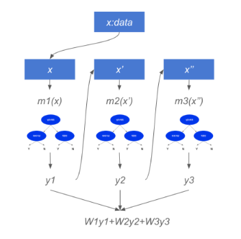
xgboost란 Boosting 은 여러가지 모델이 존재할 때 첫 번째 모델에 샘플링 된 데이터를 집어넣고 나온 결과중에서 첫 번째 모델의 에러에 대해서 분석하는 모델 2를 만든다. 또한 이 모델 2의 에러에 대해 분석하는 모델 3를 만들어 각 모델의 에러를 분석하여 향상시키는 방향으로 회귀 정확도를 향상 시킨다. 물론 XGBOOST가 회귀모델만 존재하는것은 아니다. Classification또한 XGBOOST를 이용할 수 있다.
3. 구현
1. Tensor data로 나누기 및 train test데이터 split
#데이터를 텐셔 형태로 변환해주는 클래스
class TensorData(Dataset):
  def __init__(self, x_data, y_data):
    self.x_data = torch.FloatTensor(x_data)# Double Tensor는 Float64로 변환 Float Tensor는 Float32로 변환
    self.y_data = torch.FloatTensor(y_data)
    self.len = self.y_data.shape[0]

  def __getitem__(self, index) :
    return self.x_data[index], self.y_data[index]

  def __len__(self):
    return self.len
우선 다음과 같이 텐서 형태로 데이터를 뽑아주는 함수와 클래스를 만들어 낸다.
#scikit-learn 을 이용해서 학습 데이터와 평가 데이터로 나눈다.
X_train, X_test, Y_train, Y_test = train_test_split(X,Y, test_size= 0.5) # hyper parameter 테스트 사이즈
# train데이터와 validation 데이터로 나눈다.
X2_train, X_val, Y2_train, Y_val = train_test_split(X_train, Y_train)
#학습 데이터랑 시험데이터를 배치 형태로 구축한다.
print(X2_train.shape)
print(X2_train.ndim)
print(X_val.shape)
print(Y2_train.shape)
print(Y2_train.ndim)
print(Y_val.shape)
trainsets = TensorData(X2_train, Y2_train)
trainLoader = torch.utils.data.DataLoader(trainsets, batch_size = 32, shuffle=True) # 하이퍼 파라미터 배치 사이즈

validationsets = TensorData(X_val, Y_val) #validation set
validationLoader = torch.utils.data.DataLoader(validationsets, batch_size=32, shuffle=True)

testsets = TensorData(X_test, Y_test) # 테스트 데이터들을 나눠준다.
testloader = torch.utils.data.DataLoader(testsets, batch_size = 32, shuffle=True)
그 후 scikit - learn의 train_test_split 함수를 이용하여 테스트 데이터와 훈련 데이터로 나눠준다. 그 후 shape 함수로 형태를 확인하면 다음과 같다.
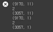
순서대로
- train data shape
- train data dimension
- validation data shape
- train label shape
- train label dimension
- validation label shape
2. Grid SearchCV 및 학습 진행
from sklearn.model_selection import GridSearchCV
from xgboost import XGBRegressor

xgb = XGBRegressor()

parameters = {
    'max_depth': [3, 7],
    'n_estimators': [500, 1000],
    'learning_rate': [0.03, 0.05, 0.07, 0.1],
    'colsample_bytree': [0.5, 0.7],
    'subsample': [0.5, 0.7, 0.8],
    'min_child_weight': [1, 5],
    'random_sate':[2],
    'n_thread': [4],
}

xgb_grid = GridSearchCV(xgb, parameters, cv=5, n_jobs=5, verbose=5)
xgb_grid.fit(X2_train, Y2_train)
scores = pd.DataFrame(xgb_grid.cv_results_)
scores[['params','mean_test_score', 'rank_test_score', 'split0_test_score','split1_test_score', 'split2_test_score']]

print(xgb_grid.best_score_)
print(xgb_grid.best_params_)
scikit learn에서 제공하는 GridSearchCV API를 이용하면 다음 미리 정의해준 파라미터 조합 중 가장 좋은 조합을 출력해줍니다.
랜덤한 넘버를 생성한 후 파라미터에 대입하고 결과를 비교해보는 방법도 있지만 가장 좋은 조합일 가능성인 파라미터는 이미 많은 사람들이 찾아놨으므로 그 중 내 모델에 잘 맞는 파라미터 조합이 무엇인지 찾는 것에는 위와 같은 방법이 효과적일 것이라는 생각에 다음과 같이 진행했습니다.
from sklearn.metrics import accuracy_score
xgbBest = xgb_grid.best_estimator_
scores = pd.DataFrame(xgb_grid.cv_results_)
pd.set_option('display.max_seq_items', None)
pd.set_option('display.max_columns', 21)
scores.info()

print(scores.sort_values(by=scores.columns[20], ascending=True).head(10))
다음과 같이 sklearn.metrics의 accuracy_score를 이용하면 xgb_grid에서 가장 좋은 점수를 낸 모델을 찾아낼 수 있습니다.
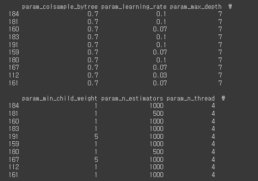
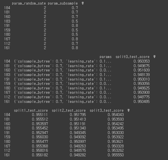
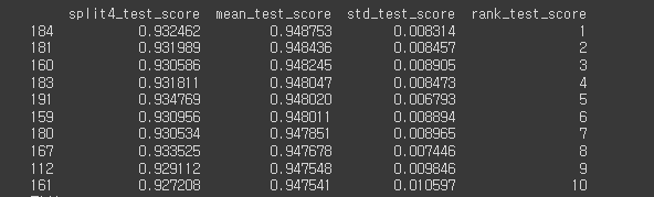
184번째 조합이 가장 좋은 점수를 냈고 이에 해당하는 파라미터 조합은 다음과 같습니다.
myxgb = XGBRegressor(objective='reg:squarederror',colsample_bytree=0.7, learning_rate=0.1, max_depth=7, min_child_weight=1, n_estimators=1000, n_thread= 4, random_state=2, subsample=0.7)
myxgb.fit(X2_train, Y2_train)
가장 좋은 조합은
- colsample_bytree = 0.7
- learnin_rate = 0.1
- max_depth = 7
- min_child_weight =1
- n_estimators =1000
- n_thread =4
- random_state = 2
- subsample =0.7
그 후 XGBRegressor()에서 제공하는 fit 메소드를 통해 학습을 진행합니다.
4. 모델 평가
Y_pred = myxgb.predict(X_test)
print(myxgb.predict(X_test))
rmse = np.sqrt(MSE(Y_test, Y_pred))
#mse = MSE(Y_test, Y_pred)
print("Test RMSE : % f" %(rmse))
#print("RMSE : % f" %(mse))
Y_true = Y_test
score = myxgb.score(X2_train, Y2_train)
score2 = myxgb.score(X_test, Y_test)
score3 = myxgb.score(X_val, Y_val)
print("Train R2 score : %f" %(score))
print("Validation R2 score : %f" %(score2))
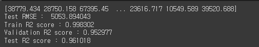
print("Test R2 score : %f" %(score3))predict메소드를 이용해서 predict결과를 만들어내고 rmse결과를 통해 오차를 확인합니다.
그 후 score메소드를 통해 R2점수를 확인하면 다음과 같습니다.
1. cross-validation 점수
다음은 train데이터에 대한 점수입니다.
from sklearn.model_selection import cross_val_score, KFold
scores = cross_val_score(myxgb, X2_train, Y2_train,cv=10)
print("Mean cross-validation score: %.2f" % scores.mean())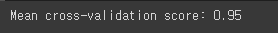
다음은 valitaion데이터에 대한 점수입니다.
valscores = cross_val_score(myxgb, X_val, Y_val,cv=10)
print("Mean cross-validation score: %.2f" % valscores.mean())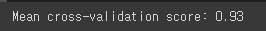
다음은 테스트 데이터에 대한 점수입니다.
testscores = cross_val_score(myxgb, X_test, Y_test,cv=10)
print("Mean cross-validation score: %.2f" % testscores.mean())
5. 모델 저장
xgboost에서 기본으로 제공하는 save_model 메소드를 통해 학습된 모델을 저장한 후 streamlit에서 사용하기 위해 저장해줍니다.
finalfilename =  'xgb_load_final2.model'
myxgb.save_model(finalfilename)
'파이썬 > ai' 카테고리의 다른 글
| [AI] Wgan-GP (Keras, TensorFlow) (1) | 2022.11.20 |
|---|---|
| [Ai, Python] Streamlit을 이용한 모델 시각화-7 (인천광역시 집 값 예측) (2) | 2022.06.26 |
| [Ai, Python] 인천광역시 집 값 예측 프로젝트 - Feature Engineering (0) | 2022.06.25 |
| [ai, python] IMDB데이터베이스의 리뷰 데이터와 RNN을 이용한 리뷰 감성 분류하기 (3) | 2022.05.29 |
| [ai, python] - Image분류 by CNN (2) | 2022.05.29 |
댓글